


Dimensionality Analysis and Why it Matters
The brain is a remarkably complex structure, capable of impressive feats, yet its mechanisms remain only partially understood. Within it lies the visual cortex, responsible for processing visual information into meaningful perceptions. Neurons in this region serve as the brain’s information processors, communicating through electrical signals. Collaboration between neurons detecting different features results in a comprehensive representation of visual input. These neurons are hierarchically organized, with lower levels processing basic features and higher levels integrating them to recognize complex objects and patterns.
The visual cortex comprises six primary layers, each with distinct roles in processing visual stimuli. While information can traverse any layer-to-layer path, consistent patterns have emerged in its trajectory. The collective behavior of neurons within this population is known as the ‘population code,’ a concept that remains elusive due to previous limitations in observing neuron structure and activity. This encoding is pivotal because incoming brain information is high-dimensional. Visual input, for instance, consists of millions of pixels with varying colors and intensities. To manage this complexity, the brain employs dimensionality reduction. This process transforms vast sensory data into a more manageable form, becoming increasingly abstract and generalized as it progresses through various brain regions. Dimensionality reduction is crucial for efficient information processing, allowing the brain to prioritize essential information while discarding less relevant details. This efficiency is vital for swift decision-making and cognitive functioning. Our paper seeks to uncover fundamental brain mechanisms by exploring the dynamics of neuron activity’s geometric portrayal across the visual cortex layers.
The dataset we are using originates from the MICrONS program, which aims to map cortical circuit function and connectivity using advanced imaging technologies. The dataset encompasses functional imaging data from approximately 75,000 pyramidal neurons, capturing individual cellular responses to diverse visual stimuli. Simultaneously, the same neural tissue underwent high-resolution electron microscopy, followed by machine learning-driven reconstruction. This process yielded an expansive anatomical connectome, including an estimated 200,000 cells and 120,000 neurons. Notably, automated synapse detection identified over 523 million synapses.
This dataset stands out for several reasons. It represents the most extensive multi-modal connectomics dataset to date, holding the distinction of being the largest in terms of minimal dimension, cell count, and detected connections up until July 2021. Furthermore, it marks the pioneering achievement of the first-ever electron microscopy reconstruction of a mammalian circuit spanning multiple functional brain areas. This dataset will allow us to conduct our analysis due to it’s innovative techniques and massive scale.
The results of this project will help contribute to the plethora of research currently happening in the computational neuroscience community. We hope our results will help inspire new techniques and models in artificial intelligence development that will make more efficient and accurate AI systems.
Results So Far
Layer Identification
Our initial project goal was to delineate the six layers within the visual cortex and understand how information flows between them. This would serve as a foundation for our analysis of neuron activity within each layer. Layers are defined based on functionality and their connections to other layers. To tackle this challenge, we devised a method: plotting the depth of a starting neuron (input) on the X-axis of a 2D graph and mapping the depth of all the neurons it outputs to on the Y-axis. By repeating this process for thousands of neurons spread throughout the visual cortex, we aimed to generate meaningful clusters of similar connections that would help us identify layer borders and comprehend the information flow across layers. For example, if we see a high concentration spot located between 100-275 microns on the X-axis and 375-575 microns on the Y-axis, we have some evidence that the neurons are following the theory and projecting from layer 2/3 to layer 5 and we can thus attempt to draw borders based on how the cluster is structured.
We gathered synapse data, encompassing approximately 9,500 neurons and over 300,000 connections, using the live server of the database. This data collection process was time-consuming, taking several weeks due to complications such as timeout issues and slow computation times. Nevertheless, once completed, we began to observe promising results. We noticed significant clustering in some of the areas we anticipated. With a margin of error, we were able to predict the locations of certain layer borders, particularly layers 2/3 and 5. By extension, we could infer the borders of layers directly adjacent to these layers and build a rough picture of where each layer lies in the cortex. Our predictions were informed by prior research as well the density of the clusters we observed.
The resulting graph is shown below:
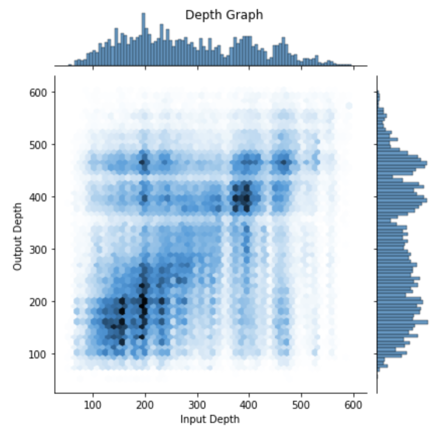
We then attempted to define borders based on the results. These borders that we identified were subsequently confirmed by the MICrONS team as they had also employed their own techniques to accomplish the same task. The result was the following values: Layer 1: 0 − 98 μm, Layer 2/3: 98 − 283 μm, Layer 4: 283 − 371 μm, Layer 5: 371 − 574 μm, Layer 6: 574 − 713 μm. μm meaning the value in microns.
The following graph shows how the border values line up with our data. While this kind of science is not “exact” and it is often difficult to define exact border values, we do see the borders lining up well with many of our clusters.

Dimensionality Analysis
Having given values to our layer structure, we moved on to our primary analysis: dimensionality. Leveraging the database, we dedicated substantial effort to extracting neuron activity in response to various stimuli, creating an activity matrix for each layer. There were many options for which stimuli to use but we ended up using six natural movies, each containing 63 frames, totaling 378 frames and each associated with electrical activity responses. These frames were presented to the mouse 10 times, allowing us to average responses for each frame and reduce some of the impact of random noise. Consequently, we obtained an activity matrix sized 378 x N, where N represents the number of neurons we observed within the layer’s borders. We then subjected this activity matrix to PCA (Principal Component Analysis).
Our current PCA model involves calculating the covariance matrix of the activity and determining the corresponding eigenvalues. When sorted in descending order, the variance for the ith principal component matches the ith eigenvalue. For instance, the first eigenvalue represents the variance explained by the first principal component, or dimension. Thus, the eigenvalues, also called the eigenspectrum, of each layer give us insight into the neuron population’s geometric portrayal.
We are currently in the process of conducting this analysis so we are not prepared to draw any definite conclusions; however we do have some preliminary results that give us hope that we will be able to understand some key characteristics of how the neurons process the stimuli.
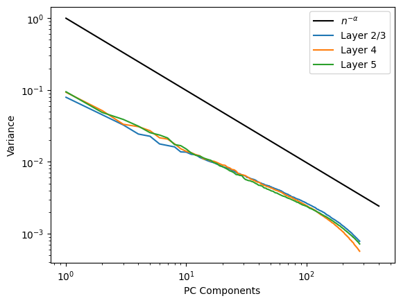
This graph represents the results from layers 2/3, 4, and 5. Layers 1 and 6 are not represented due to the lack of sufficient neurons. What we can see is that each layer shows an overlapping variance decay. This could mean that there is something truly special about this rate of change. Previous papers attempting to accomplish the same tasks have proven mathematically that if variances decay more slowly than a power law n-𝛼 with exponent α = 1 + 2/d, where d is the dimension of the input ensemble, then the space of neural activity must be non differentiable or not smooth. A smooth neural activity allows similar images to evoke similar responses and this is often what we observe empirically. We have included the line n-𝛼 as as point of reference so you can see how this seems to line up. Our observed decay seems to be a bit slower than expected however there are an abundance of unaccounted for factors that we must take care of before drawing conclusions. The main one being that we have not removed all of the neural activity that is a result of movement in the mouse. The neurons in the visual cortex are primarily responsible for processing visual information but they also respond to a variety of other stimuli such as motor movement so to make sure that we are isolating a single variable, we must implement techniques to remove this variable.
What’s Next?
As stated in the results section, we are next going to attempt to remove the impact that motor movement activity has on the visual cortex neurons. There are a few ways to do this one of which involves using a different method of PCA called cvPCA (cross-validated PCA), however we have not evaluated which we will pursue yet. In addition to analyzing dimensionality across each layer, we are also interested in examining dimensionality in other distinct areas of the visual cortex to see if the results change and if they do, explore why that would be the case.
Authors: Riley Jenum, Alessandro Pagan, Barbara Karwowska, Emma Anastassova


